Code
import os
import numpy as np
import matplotlib.pyplot as plt

from maxrf4u import DataStack, multi_plot
import skimage.exposure as skeThe whole point of doing all this is of course to be able to communicate the results of data processing in as rich a manner as possible. We have saved the calculated element maps in our datastack file. With the multi_plot() function one can create an overview plot with just a few lines of of code.
import os
import numpy as np
import matplotlib.pyplot as plt
from maxrf4u import DataStack, multi_plot
import skimage.exposure as skeos.chdir('/home/frank/Work/Projecten/DoRe/viz/raw_nmf')
datastack_file = 'RP-T-1898-A-3689.datastack'
ds = DataStack(datastack_file)
elements = ds.read('nmf_elements')
element_maps = ds.read('nmf_elementmaps')
element_maps_histeq = [ske.equalize_hist(m) for m in element_maps]
fig, axs = multi_plot(*element_maps_histeq, titles=elements)
fig.suptitle('histogram equalized element maps')
plt.tight_layout()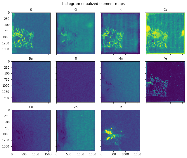
Now I would like to share and explore this result with my colleagues and the rest of the world. Of course, one could save this plot in a low resolution overview image and share by email, or perhaps create a zip folder with high resolution images and send by Wetransfer. Rather unsatisfactory, clumsy, inefficient. In my experience, when exploring data each new thought requires yet another view of the same data. In some cases this is just a matter of zooming in to a specific location on the map, in other cases one might need to adjust contrast, mark locations etcetera. All of this is easy when one knows how to use Python and is sitting behind the same computer. However, I am aware that most of my colleagues can not program Python, and have other problems in life that they would like to solve first.
For effective data exploration within interdisciplinary teams, being able to easily create interactive web based visualizations is paramount.
In the scientific Python community the need for interactive web based data visualization has since long been well understood. In these last years a rich ecosystem of open source web visualization tools has been developed. Two important Python packages that allow easy creation of interactive web dashboards are ipywidgets and ipyleaflet. My code here is makes use of these packages.
Of course, one can only create web visualizations if one has the possibility to directly publish content on the web. Github offers free webhosting for nerds. These documentation pages you are reading are published via github. However, github is a version control system for code and not suitable to publish large amounts of image data. Better suited is cloud storage. In my case I acquired cloud storage from backblaze.com. The price for storing files is very cheap: $0.005 GB/Month. Cloud storage is organized in so-called buckets. Files within those buckets can be loaded into web pages. A convenient way to upload files to a web bucket is to mount the bucket into the computer’s file system using a command line tool called rclone.
Enough talk for now. Below I will show you how to create an interactive visualization. Starting point is the histogram equalized element maps for the eleven elements.
from maxrf4u import DataStack, multi_plot
import skimage.exposure as skedatastack_file = 'RP-T-1898-A-3689.datastack'
ds = DataStack(datastack_file)
elements = ds.read('nmf_elements')
element_maps = ds.read('nmf_elementmaps')
element_maps_histeq = [ske.equalize_hist(m) for m in element_maps] # improve contrastLet’s start by preparing standard filenames for the jpeg images that will be used in the visualization using the make_filenames() function.
from maxrf4u import make_filenamesobjnr = 'RP-T-1898-A-3689'
viztype = 'histeq_elementmap'
ext = 'jpg'
filenames = make_filenames(objnr, viztype, elements, ext)
filenames['RP-T-1898-A-3689_histeq_elementmap_S.jpg',
'RP-T-1898-A-3689_histeq_elementmap_Cl.jpg',
'RP-T-1898-A-3689_histeq_elementmap_K.jpg',
'RP-T-1898-A-3689_histeq_elementmap_Ca.jpg',
'RP-T-1898-A-3689_histeq_elementmap_Ba.jpg',
'RP-T-1898-A-3689_histeq_elementmap_Ti.jpg',
'RP-T-1898-A-3689_histeq_elementmap_Mn.jpg',
'RP-T-1898-A-3689_histeq_elementmap_Fe.jpg',
'RP-T-1898-A-3689_histeq_elementmap_Cu.jpg',
'RP-T-1898-A-3689_histeq_elementmap_Zn.jpg',
'RP-T-1898-A-3689_histeq_elementmap_Pb.jpg']A next step is to create an standard image upload directory object and upload the images to the cloud storage. This is done with the UploadDir() function and .imsave() method.
from maxrf4u import UploadDirbucket_url = 'https://f002.backblazeb2.com/file/dore-viz'
mount_dir = '/media/frank/b2/dore-viz/'
uplink = UploadDir(mount_dir, objnr, bucket_url, subdir='images')Created online images folder: https://f002.backblazeb2.com/file/dore-viz/RP-T-1898-A-3689/imagesimg_urls = uplink.imsave(element_maps_histeq, filenames)Saving 11 images to folder: https://f002.backblazeb2.com/file/dore-viz/RP-T-1898-A-3689/images
https://f002.backblazeb2.com/file/dore-viz/RP-T-1898-A-3689/images/RP-T-1898-A-3689_histeq_elementmap_S.jpg
https://f002.backblazeb2.com/file/dore-viz/RP-T-1898-A-3689/images/RP-T-1898-A-3689_histeq_elementmap_Cl.jpg
https://f002.backblazeb2.com/file/dore-viz/RP-T-1898-A-3689/images/RP-T-1898-A-3689_histeq_elementmap_K.jpg
https://f002.backblazeb2.com/file/dore-viz/RP-T-1898-A-3689/images/RP-T-1898-A-3689_histeq_elementmap_Ca.jpg
https://f002.backblazeb2.com/file/dore-viz/RP-T-1898-A-3689/images/RP-T-1898-A-3689_histeq_elementmap_Ba.jpg
https://f002.backblazeb2.com/file/dore-viz/RP-T-1898-A-3689/images/RP-T-1898-A-3689_histeq_elementmap_Ti.jpg
https://f002.backblazeb2.com/file/dore-viz/RP-T-1898-A-3689/images/RP-T-1898-A-3689_histeq_elementmap_Mn.jpg
https://f002.backblazeb2.com/file/dore-viz/RP-T-1898-A-3689/images/RP-T-1898-A-3689_histeq_elementmap_Fe.jpg
https://f002.backblazeb2.com/file/dore-viz/RP-T-1898-A-3689/images/RP-T-1898-A-3689_histeq_elementmap_Cu.jpg
https://f002.backblazeb2.com/file/dore-viz/RP-T-1898-A-3689/images/RP-T-1898-A-3689_histeq_elementmap_Zn.jpg
https://f002.backblazeb2.com/file/dore-viz/RP-T-1898-A-3689/images/RP-T-1898-A-3689_histeq_elementmap_Pb.jpgNow that we have these images available online, we can build the interactive ‘gridbox’ visualization with the make_gridbox_widget() function, and save the the result as an html webpage with the .export_interactive_html() method.
from maxrf4u import make_gridbox_widgetgridbox = make_gridbox_widget(img_urls, titles=elements)uplink.export_interactive_html(gridbox, viztype='histeq_elementmap');Saving interactive html to cloud storage...
Click link to load the interactive visualization (opens a separate page).
https://f002.backblazeb2.com/file/dore-viz/RP-T-1898-A-3689/html/RP-T-1898-A-3689_histeq_elementmap.htmlClick link to load the interactive visualization (opens a separate page).
def export_element_maps(
    datastack_file, output_dir:NoneType=None, histeq:bool=True
):
Save element maps as separate png images.
def make_gridbox_widget(
    img_urls, titles, shape:NoneType=None
):
Creates multi-image interactive synchronized viewer.
def make_filenames(
    objnr, viztype, titles, ext
):
Creates standard filenames.
Returns: filenames
def UploadDir(
    mount_dir, objnr, bucket_url, subdir:str='images'
):
Creates a standard upload (image) directory object.