from maxrf4u import calibrate, DataStackCalibration
Find the Compton peak first
Inconveniently, MA-XRF data does not always include information about the energy calibration of the spectra. Although it is clear that the channel energies will roughly range between zero and the tube voltage, we need more precise numbers for the upcoming calculations. Thus, a very first step in the data analysis is to obtain a precise energy calibration in keV units (kilo-electron-Volt) for a given dataset. Fortunately, XRF spectra, (at least for drawings), typically have two clearly recognizable features that allow for energy calibration of the detector channels.
Two steps
The automatic precise energy calibration is done in two steps.
In the first step the dominant broad Compton peak is observed in the sum spectrum. The position of this peak can not be used for the calibration directly due to an unknown (detector angle specific) Compton shift, but it serves as a landmark. Right next to the Compton peak a small peak is found. In our lab an x-ray tube with a Rhodium anode is used. This peak can now be attributed to elastic scattering of the strong Rhodium K-alpha emission peak present in the x-ray tube spectrum at 20.21 keV.
In the second step of the calibration process the iron K-alpha emission peak is located in the max spectrum. Essentially all artifacts like paper contain iron, with a known strong emission K-alpha line at 6.403 keV.
As a first requisite step in any further data analysis the function calibrate() is called. The user is prompted to inspect and save the result.
x_keVs = calibrate('RP-T-1898-A-3689.datastack', tube_keV=40)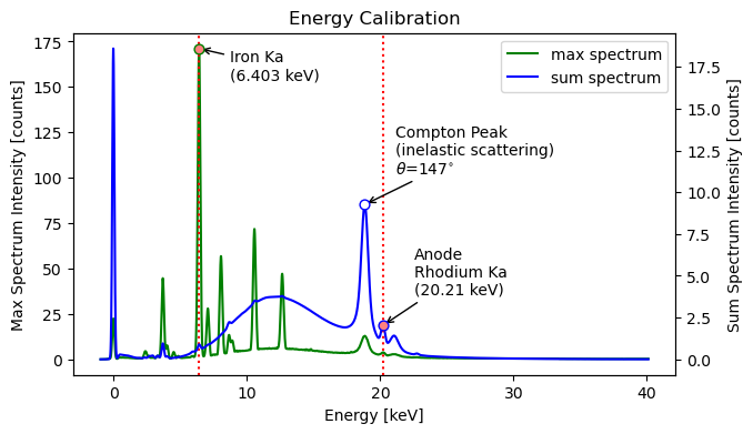
Write instrument energy calibration to datastack file [y/n]? y
Writing channel energies (keV) to: RP-T-1898-A-3689.datastack
Also writing instrument Compton anode peak energy (keV) to: RP-T-1898-A-3689.datastack
In further analysis our stored energy calibration can now be accessed using the .read('maxrf_energies') method which returns an array with 4096 energy values.
ds = DataStack('RP-T-1898-A-3689.datastack')
x_keVs = ds.read('maxrf_energies')

print('Energies: ', x_keVs)
print(f'Number of energy channels: {len(x_keVs)}')
Energies: [-0.98188629 -0.97185221 -0.96181812 ... 40.08763102 40.09766511
40.1076992 ]
Number of energy channels: 4096Now that we have an energy calibration, we can move to the next step in our data analysis…
FUNCTIONS
compton_shift
def compton_shift(
    keV_in, theta
):
Compute Compton shift for photon energies keV_in and scatter angle theta.
Assuming single scattering.
Returns: keV_out
find_instrument_peaks
def find_instrument_peaks(
    y_sum, prominence:float=0.03, tube_keV:int=40
):
Locate key instrument peaks:
      1) left hand sensor peak index
      2) anode Compton peak index
      3) right hand (rhodium) anode Ka peak index

      in sum spectrum `y_sum`.
Assumes anode material is rhodium, and Compton peak energy is first peak below (uncalibrated) 20 keV, based on tube keV.
Returns: [left_peak_i, compton_peak_i, right_peak_i]
detector_angle
def detector_angle(
    keV0, keV1
):
Calculate detector scatter angle theta (degrees)
From Compton peak energy keV0 and anode energy keV1, assuming a single scattering event.
Returns: theta (degrees)
calibrate
def calibrate(
    datastack_file, anode:str='Rh', prominence:float=0.03, tube_keV:int=40, auto_write:bool=False,
    manual_range:NoneType=None
):
Automatic two step energy energy calibration.
In step 1 a preliminary calibration is done assuming that the
sensor peak is located at 0 keV and the Rhodium anode Ka peak is next to it’s high and broad Compton scattering peak in the sum spectrum.
This preliminary calibration the enables the identification of Fe_Ka peak in the max spectrum and a second precise calibration.
Asks user confirmation to store energy calibration in datastack file.
Returns: x_keVs