Plotting Kendrick plots

Can’t wait to make our first Kendrick plot!

Let’s see if we can now explore the mass spectral data in our cached raw file. However, before creating a Kendrick plot let’s take a look at the (centroided and time integrated) positive and negative mode mass spectra. This can be done conveniently with a bit of matplotlib code.

from kendrick import read_raw, centralize 
import matplotlib.pyplot as plt
import os 
import numpy as np

raw_file = '/home/frank/.cache/fairdatanow/asap-data/2025 Théo-Fany Lange - the dutch method/xcalibur raw data files/Matt_Joana_100-24-1_01.RAW'

df_pos, df_neg = read_raw(raw_file) 
df_total_pos = centralize(df_pos)
df_total_neg = centralize(df_neg)

fig, ax =plt.subplots(figsize=[12, 8])

xlabel, ylabel = df_total_pos.columns
x_pos, y_pos = df_total_pos.values.T
x_neg, y_neg = df_total_neg.values.T
title = f'{os.path.basename(raw_file)}'

ax.vlines(x_pos, np.zeros_like(y_pos), y_pos, color='firebrick', label='positive mode (+)')
ax.vlines(x_neg, -y_neg, np.zeros_like(y_neg), color='royalblue', label='negative mode (-)')
ax.set_xlabel(xlabel)
ax.set_ylabel(ylabel) 
ax.set_title(title)
ax.legend();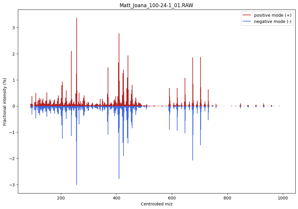

Kendrick plots are simply another representation of the same data. From the centroided m/z values we can compute the Kendrick mass and the Kendrick mass defect with the compute_kendrick_mass_and_defect() function.

from kendrick import compute_kendrick_mass_and_defect

mz_pos = df_total_pos['Centroided m/z'].values 
inty_pos = df_total_pos['Fractional intensity (%)']
km_pos, kmd_pos = compute_kendrick_mass_and_defect(mz_pos) 

mz_neg = df_total_neg['Centroided m/z'].values 
inty_neg = df_total_neg['Fractional intensity (%)']
km_neg, kmd_neg = compute_kendrick_mass_and_defect(mz_neg) 

fig, ax = plt.subplots(figsize=[12, 8]) 
thres_pos = 0.0001
s_pos = 500

thres_neg = 0.0001
s_neg = 800

ax.set_ylim([-0.05, 0.6])
ax.set_xlim([0, 1200])
ax.scatter(km_neg[inty_neg > thres_neg], kmd_neg[inty_neg > thres_neg], s=s_neg*inty_neg[inty_neg > thres_neg], alpha=0.8, color='royalblue', label='negative mode (-)')
ax.scatter(km_pos[inty_pos > thres_pos], kmd_pos[inty_pos > thres_pos], s=s_pos*inty_pos[inty_pos > thres_pos], alpha=0.5, color='darkred', label='positive mode (+)')

ax.set_xlabel('Kendrick precise mass (KM)')
ax.set_ylabel('Kendrick mass defect (KMD)')
ax.set_title(f'Kendrick plot for {os.path.basename(raw_file)}')
ax.legend();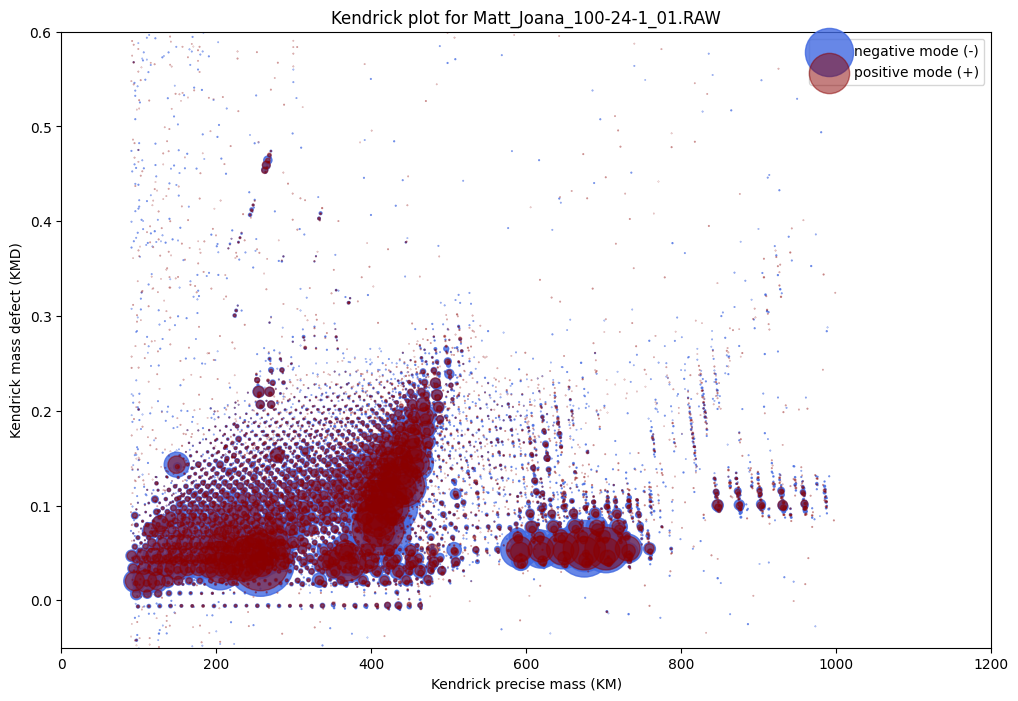

This Kendrick plot looks somewhat similar to the excel version by Wim. We need to figure out the reasons for these differences…

Functions

---

source

compute_kendrick_mass_and_defect

def compute_kendrick_mass_and_defect(
    mz, monomer:str='CH2', offset:float=0.6
):

Compute Kendrick precise mass for array mz.

Default monomer is ‘CH2’.

It is not clear to me why the offset by Wim is chosen 0.6.

Reurns: km, kmd